After my two recent posts on modeling friction and kinematic clutches, I felt as though I had missed out on some opportunities to explain how these kinds of kinematic models fit into the big picture of transmission modeling. So for this post, I'd like to take a step back and not focus exclusively on the internal workings of components, but to show how these kinds of techniques can be used to model complete subsystems.

I should also point out that all the source code used in this example and my previous post about kinematic clutches is now available on GitHub in the xogeny/Kinematics repository and is distributed under a Creative Commons Attribution 3.0 Unported License.

Transmission Function

Just as with the two previous posts, the models here will be what I would call "functional" models. That is to say that the models should reproduce the function of (in this case) a transmission but without the need to specify lots of design details.

The main function of the transmission is to act as a gear to allow the engine and/or electric motors to generate torque in a speed range that leads to efficient energy conversion. However, since the speed of the vehicle changes over a wide range, it is necessary for the "gear ratio" of the transmission to change in some manner in order to keep the engine/motors operating at their most efficient speeds.

However, a transmission is not always "in gear". For example, when you put the transmission in neutral, the transmission disconnects the engine from the driveline. Also, in an automatic transmission the effects of the torque converter are felt whenever the bypass clutch is disengaged. In this post, our functional transmissions will provide the functionality of neutral, but not the functionality of the torque converter.

The architecture for our transmission model looks like this:

partial model PartialTransmission
  Modelica.Mechanics.Rotational.Interfaces.Support support "Transmission housing";
  Modelica.Mechanics.Rotational.Interfaces.Flange_b output_shaft "Output shaft";
  KinematicClutch kinematicClutch(shift_time=engagement_time, start_engaged=start_engaged) "Provides neutral functionality";
  Modelica.Mechanics.Rotational.Interfaces.Flange_a input_shaft "Input shaft";
  Modelica.Blocks.Interfaces.BooleanInput engage "Signal transmission to engage";
  parameter Modelica.SIunits.Time engagement_time;
  parameter Boolean start_engaged=true;
protected
  replaceable PartialGear gear(final useSupport=true);
equation
  connect(gear.support, support);
  connect(gear.flange_b, output_shaft);
  connect(kinematicClutch.flange_b, gear.flange_a);
  connect(kinematicClutch.flange_a, input_shaft);
  connect(kinematicClutch.command, engage);
end PartialTransmission;

A simple summary of this model is that it includes a gear box and an engagement clutch. The engagement clutch is the KinematicClutch from my previous post and is controlled by the Boolean input signal engage, which is used to signal the transmission to engage (i.e., shift out of neutral).

Note that the gear model is replaceable. This is, in fact, why the entire model is partial. The model is useless unless an actual gear model is specified.

As an aside, you may also notice that the gear model is in a protected section. This is by design. In order to make this model into a non-partial version, a gear model must be specified. Because the gear model is protected, such a change can only be made by extending from this class. It may seem like a minor point, but this is actually a useful and important technique for model management. Without this "pattern", people might drag this model down into a diagram and then modify the gear model. For reasons that I won't really get into now (perhaps a topic for a future post), this can create some serious headaches for managing complex models. By making the gear model protected, it forces users to create a new named model, not just some "anonymous instance". But I digress, back to the topic at hand.

We will use this model as the foundation for two models in this post, a continuously variable transmission (CVT) model and a step ratio transmission model.

The Gear

Most of the interesting behavior in our transmission will come from a gear model. We already saw that our PartialTransmission model specifies a way to specify the particular kind of gear model we want in the transmission. The interface for the model is defined by the PartialGear model and looks like this:

partial model PartialGear "Base class for a variety of kinematic gear models"
  extends Modelica.Mechanics.Rotational.Interfaces.PartialElementaryTwoFlangesAndSupport2;
protected
  Real R "gear ratio";
  Modelica.SIunits.Angle phi_a "Angle between left shaft flange and support";
  Modelica.SIunits.Angle phi_b "Angle between right shaft flange and support";
equation
  phi_a = flange_a.phi - phi_support;
  phi_b = flange_b.phi - phi_support;
  der(phi_a) = R*der(phi_b);
  0 = R*flange_a.tau + flange_b.tau;
end PartialGear;

This is almost an exact copy of the IdealGear model from the Modelica Standard Library (MSL). This model is partial because the gear ratio, R, is declared in the model, but there is no equation for it. In order to create a non-partial implementation, it is necessary to extend this model and provide a definition for the behavior of R

As another aside, one thing to note here is the presence of a support element to represent the housing of the gear box. Far too often, people overlook the effects of reaction torques in drivelines so I always make it a point to explicitly include the transmission housing, even if I simply connect it to a mechanical ground.

Continuously Variable Gear

If we wish to create a CVT model, the only thing we really need to do is create a continuously variable gear model. At first glance, the following model might appear to suffice:

model CVT_Gear "A continuously variable gear"
  extends Modelica.Mechanics.Rotational.Icons.Gear;
  extends Kinematics.Interfaces.PartialGear;
  Modelica.Blocks.Interfaces.RealInput ratio "Desired gear ratio";
equation
  R = ratio;
end CVT_Gear;

However, there is a subtle problem here. With this definition, we have no assurances about the smoothness of the input signal ratio. Specifically, it might not be smooth. This means someone could command a step change in ratio. This is a problem because in our previous base class, PartialGear, we had the following line:

der(phi_a) = R*der(phi_b);

It turns out that in most cases this line will be differentiated as part of the index reduction process. If so, it will typically be necessary to differentiate R with respect to time.

To handle cases where index reduction may be performed, we ensure the necessary smoothness directly in our model by using a first order filter on the input signal. This is actually well aligned with the function of the CVT since CVTs cannot support step changes in ratio anyway. So our modification will not only provide the mathematical assurances we need, but will also mimic the functional behavior of the CVT. The resulting model looks like this:

model SmoothCVT_Gear "A continuously variable gear with smoothing"
  extends Modelica.Mechanics.Rotational.Icons.Gear;
  extends Kinematics.Interfaces.PartialGear;
  parameter Modelica.SIunits.Time tau "Time constant for ratio change";
  Modelica.Blocks.Interfaces.RealInput ratio "Desired gear ratio";
initial equation
  R = ratio;
equation
  tau*der(R) = ratio-R;
end SmoothCVT_Gear;

where tau represents the time constant for the CVT shifting process. Once we have this SmoothCVT_Gear component model, we can combine it with our PartialTransmission model for a complete (non-partial) CVT model:

model CVT_Transmission "A transmission with a continuous variable gear ratio"
  extends Interfaces.PartialTransmission(redeclare
  Kinematics.Components.SmoothCVT_Gear gear(tau=tau));
  Modelica.Blocks.Interfaces.RealInput ratio "Desired gear ratio";
  parameter Modelica.SIunits.Time tau "Time constant for ratio change";
equation
  connect(gear.ratio, ratio);
end CVT_Transmission;

Voila! A continuous variable transmission model that includes all the functional behavior (neutral, engagement time, ratio change dynamics) but without the need to specify any design details.

Step Ratio Gear

To provide yet another example of defining functional behavior kinematically, let's consider the behavior of the more common step ratio transmission model. This is the kind of behavior you see in most cars (either automatic or manual). In this case, the transmission cannot take on just any gear ratio but is constrained to a relatively small number of specific ratios.

Again, we start by extending the PartialGear model:

model StepRatio_Gear "A step ratio gear model"
  extends Modelica.Mechanics.Rotational.Icons.Gear;
  extends Kinematics.Interfaces.PartialGear;
  parameter Real ratios[:] "Discrete gear ratios";
  Modelica.Blocks.Interfaces.IntegerInput gear "Desired gear";
  parameter Modelica.SIunits.Time shift_time "Time to shift gears";
protected
  Modelica.SIunits.DampingCoefficient dR "Rate of ratio change";
  Modelica.SIunits.Time start_time "Start of last shift";
initial equation
  R = ratios[gear];
  dR = 0;
  start_time = time-2*shift_time;
equation
  der(R) = if time<=start_time+shift_time then dR else 0;
  when change(gear) then
start_time =  time;
dR = (ratios[gear]-R)/shift_time;
  end when;
  assert(gear>=1 and gear<=size(ratios,1),
         "Selected gear is outside valid range of 1-"+String(size(ratios,1)));
end StepRatio_Gear;

The interface to this model has three elements:

parameter Real ratios[:] "Discrete gear ratios";
Modelica.Blocks.Interfaces.IntegerInput gear "Desired gear";
parameter Modelica.SIunits.Time shift_time "Time to shift gears";

The ratios array contains the set of discrete ratios that the transmission can support. The gear input signal is an integer signal that indicates which of the specified gear ratios is being requested. Finally, the shift_time is another parameter related to the internal dynamics. As we have seen repeatedly with these kinematic models, the timing of the events (shifting, engagement, etc.) are, once again, prescribed by a parameter.

You may notice the presence of the assert statement in the model. This ensures that the input values for gear stay within the expected range of 1-N (where N is the number of discrete gear ratios). Should the input stray outside that range, an error will be generated by this assert statement. The assert statement is an extremely useful and important part of making models that are robust and fail gracefully when inputs or variables exceed their expected limits.

You will see many similarities between the implementation of this model and the KinematicClutch model. Whereas the SmoothCVT_Gear model used a first order response to change from one ratio to another, the KinematicClutch and StepRatio_Gear models slew linearly.

As with the CVT case, creating a complete transmission model is simply a matter of extending the PartialTransmission model:

model StepRatioTransmission "A step ratio transmission"
  extends Interfaces.PartialTransmission(redeclare
  Kinematics.Components.StepRatio_Gear gear(shift_time=shift_time, ratios=ratios));
  parameter Modelica.SIunits.Time shift_time "Time to shift gears";
  parameter Real ratios[:] "Discrete gear ratios";
  Modelica.Blocks.Interfaces.IntegerInput gear_cmd "Desired gear";
equation
  connect(gear.gear, gear_cmd);
end StepRatioTransmission;

Backward Driven

Another benefit of this approach that I completely failed to mention when discussing the KinematicClutch models was the ability to do backward driven models.

In the world of drive cycle simulation, there are two different "flavors" of models. The first are "forward driven", where the solution process starts with specifying the driver pedal demand and then, from there, the engine torque is computed, which gives the output torque of the transmission, which then allows the acceleration (and therefore speed) of the vehicle to be computed. However, because the speed of the vehicle is actually specified for standard drive cycles, a "backward driven" approach is often used where the speed of the vehicle is known and from there the vehicle acceleration is computed, which then leads to the calculation of the required output torque from the transmission and this allows the engine torque to be calculated, which can then be mapped to the driver pedal demand.

The beauty of these kinematic models is that they can be used for both forward and backward driven use cases without any change to the transmission model!

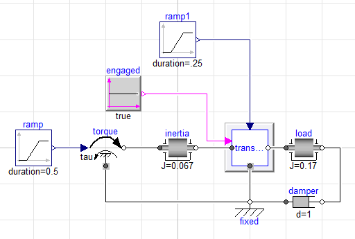
Consider the following forward driven model:

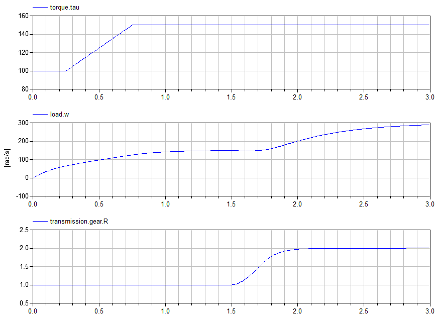
Note here how the torque applied to the transmission is explicitly specified. From such a simulation, we can then plot the resulting response for the load inertia:

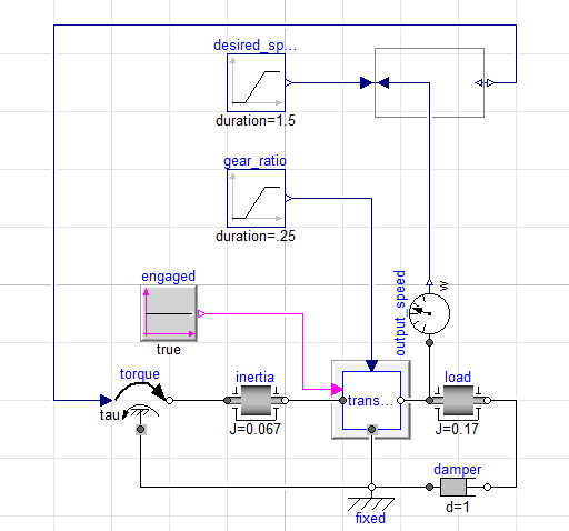
Here is a backward driven version of the same model:

Now, to make this a backward driven model we only need to introduce a sensor to measure speed response, a block to indicate our desired response and an InverseBlockConstraints block and we now have a backward driven model. The essential point here is that we did not change the physical model at all, only the way that the input torque was specified.

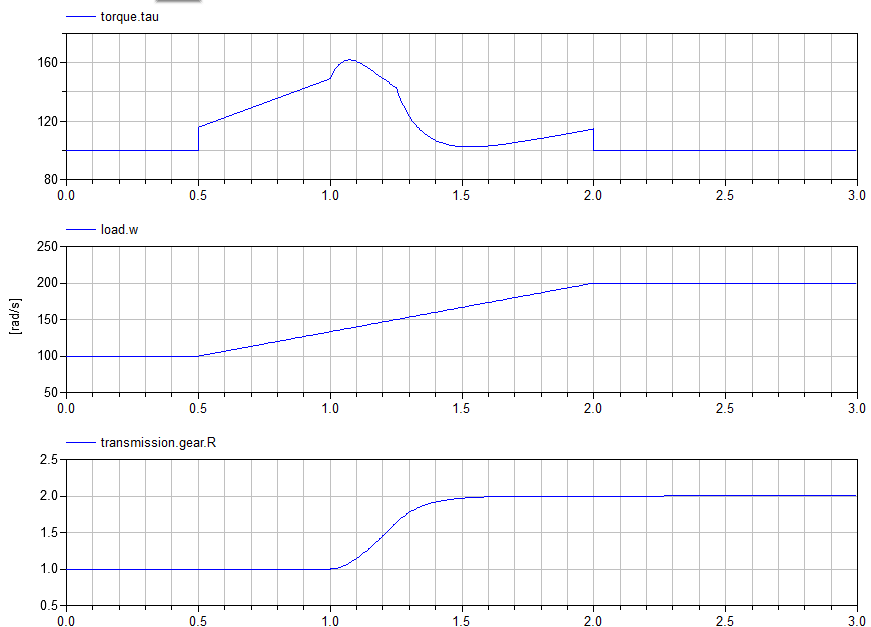
We can see in the simulation results that the kinematic constraint (the desired response) was met perfectly and the torque required to achieve this response is computed for us:

Reaction Torques

If you have built models like this using a "block diagram" approach (e.g. in Simulink), it may seem like we've done a bit more work than expected here in smoothing and slewing these ratio changes. At first glance, it may not be obvious why this is necessary.

There are two points to make here. First, keep in mind that because of the object-oriented nature of Modelica most of the heavy lifting (dealing with smoothness of the ratio change) really only needs to be done once for each type of model and can be encapsulated within the transmission model as we have shown.

Second, and more importantly, these models are based on conservation principles. Specifically, we are assured conservation of angular momentum in these models. This, in turn, means that our simulation results will always yield all the appropriate reaction torques in the model.

When specifying behavior in terms of kinematic constraints, you are formulating implicit, rather than explicit, equations for the torques involved. In a sense, you are saying "compute the torque such that this kinematic relationship will always be true". This is actually quite powerful because it means that you can then go back after a simulation and examine how much torque the KinematicClutch had to be able to generate in friction or how much torque the input shaft of the transmission needs to withstand for a given maneuver.

There are actually several different reaction torques of interest in the examples shown. First, the KinematicClutch model will compute how much torque is necessary in order to engage the clutch and keep it engaged (also called the "clutch torque capacity"). The gear models (e.g. CVT, step ratio) will compute the amount of torque the transmission will have to handle during a shift. In particular, the so called "inertia torque", which results from having to speed up or slow down rotating elements will be computed in our approach. For a backward driven model, the torque required to achieve the desired response is a form of "reaction torque" and will be computed for us. Finally, the reaction torque on the transmission housing (due to the kinematic constraint that "grounds" it) is also computed. This gives you a sense of the kind of loadings that the powertrain mount system will have to handle.

All this comes at minimal cost because of the ubiquitous application of conservation principles.

Conclusion

In conclusion, the use of kinematic constraints is not restricted to component models but can be a very effective tool in the early stages of a system engineering driven process to predict the behavior of systems and subsystems without the need for design information.

Since these kinds of functional models are often used for system level design and verification processes in system engineering, this gives kinematic models two big advantages. First, they can successfully avoid requiring design information (which would mean going deeper down the system engineering V than is strictly required at this point) and it means that the models can yield key requirements (torque capacity of clutches, stresses in shafts, etc.) that must be cascaded down the design side of the V for the next step of the process. This not only allows options and concepts to be quickly explored but can be used to formulate requirements that will ultimately drive the design process.

As mentioned previously, the source code for all of the models described in this post is available on GitHub in the xogeny/Kinematics repository and is distributed under a Creative Commons Attribution 3.0 Unported License.