Note: Javascript is required on this page to properly typeset equations.

This is part two of my discussion on clutch modeling. You might want to read part one, but I don't think it is strictly necessary.

Functional Models vs Predictive Models

In this article, I'm going to show an interesting way to model clutches in Modelica. More specifically, I'm going to show how to build a functional model of a clutch.

This distinction requires some preliminary explanation. If you want to understand how the physical design (geometry, materials, etc) of a clutch influences its behavior but you don't want to go to the time, trouble and expense of actually fabricating a prototype of that clutch (or the subsystem it belongs to) then you typically use a mathematical model to try and predict how the real clutch will behave. I refer to such models as predictive models because, obviously, the objective of the model is to predict behavior without having a physical version. It is essential that a predictive model accurately captures the effects of design changes.

But there are many applications where you really don't need a predictive model. In some cases, you simply want to build component models that behave in some reasonable way. In those cases, you want models that capture the function of the component. These models are often much simpler because they do not have to consider the effects of design.

As an aside, when I build predictive models of complex systems I typically start with functional models of everything in the system and simulate the system to make sure that I have properly captured the functional descriptions of the various constituents. If all the components function properly, then I can validate the system (components, connections, etc) by checking that the system as a whole functions properly. Once I am convinced I have architected my model correctly, I can then refine the model to add predictive details as needed, checking along the way that the overall function of the system is largely preserved.

Behavior

The Function of a Clutch

But, as I mentioned before, the goal of this article is to talk about functional clutch modeling. To make any progress here, we first need to define the function of a clutch. Let's bring back the simple diagram from part one of this article:

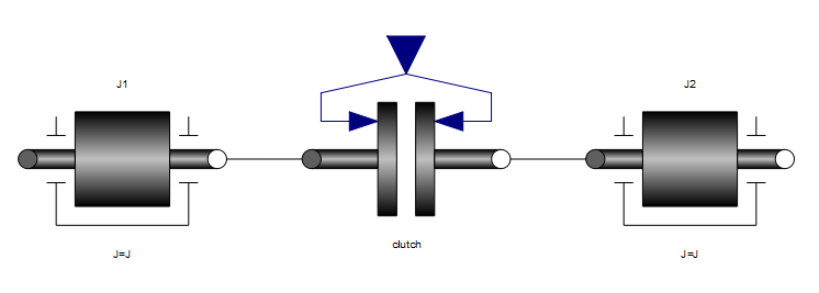
From a functional standpoint, the goal of the clutch is to get the two inertias to rotate with the same speed when the clutch is engaged. When the clutch isn't engaged, the clutch should (ideally) exert no influence on the two inertias. This is, of course, an extremely (if not overly) simple model of a clutch. But it is also useful in circumstances where either you are not concerned about the physical behavior of the clutch or you can safely assume that someone else in the design process will build a clutch (and its associated control system) to perform as desired.

Prescribing Clutch Response

The key here is that rather than describing the behavior of a clutch in terms of explicit equations for the friction, e.g.

\[ \tau = c_{geo} \mu(\Delta \omega) F_n \]

we instead describe the behavior of the clutch in terms of how it should respond functionally. Before we can do that, we need to identify the four distinct "modes" of behavior.

For simplicity, we will name these models "Engaging", "Engaged", "Disengaging", "Disengaged". Let's first go through each of these to understand what we expect the clutch to do in each of these phases. For simplicity, we'll start with "Disengaged" and work our way through the other options:

• Disengaged: Simply put, when the clutch is disengaged it does nothing. This means there is no torque acting on either clutch plate. Mathematically, \(\tau = 0\).

• Engaging: When the clutch is engaging, we prescribe a trajectory for the relative speed across the clutch. This is why I call this kind of clutch a kinematic clutch, because it imposes a kinematic constraint on the system. Mathematically, in this mode the behavior is \(\omega = f(t)\)

• Engaged: When the clutch is engaged (i.e. the relative speed across the plates is zero), we simply ensure that it stays that way, i.e. \(\omega = 0\)

• Disengaging: We could assume that the clutch immediately returns to the Disengaged mode (i.e. \(\tau = 0\)), but this isn't very realistic. Instead, what is slightly more in line with the function of the clutch is to simulate the effect of the friction "letting go" (i.e. having a gradually diminishing influence). So for this case, we prescribe the a trajectory for the torque such that it gradually drops to zero. Mathematically, we can express this as \(\tau = f(t)\).

In addition to these four modes, we need to consider why the clutch moves from one mode to another. The various transitions we will consider are:

• Disengaged → Engaging: This should occur because the clutch was commanded to engage. While a normal clutch "command" would be a hydraulic pressure or force, for a kinematic clutch the command is simply a Boolean flag indicating whether the intent is for the clutch to be engaged or disengaged. If the clutch is disengaged and the command requests that it be engaged, we make the transition from Disengaged to Engaging.

• Engaging → Engaged: After the command to engage the clutch has been sent, the relative speed across the clutch plates will eventually reach zero. Once it does, the clutch is said to be Engaged.

• Engaging/Engaged → Disengaging: If the clutch is in the process of engaging and the engagement command switches to a "disengage" command, we need to "back out" of our engagement (i.e. switch to the Disengaging mode). Technically, it doesn't matter whether the clutch was Engaging or simply Engaged when the command to disengage is received, the effect will be the same.

• Disengaging → Disengaged: While disengaging, we are prescribing the torque across the clutch. As was mentioned previously, the intent is that the torque eventually reaches zero. When that happens, we can consider the disengagement complete and move to the Disengaged state again.

Functional vs. Physical

One thing you have to watch out for when you prescribe the physical response of a system is that it may not actually make physical sense. For example, a clutch relies on friction to achieve its function. As such, the torques that it produces are always in opposition to the direction of motion. Specifically, when you push together the two clutch plates, friction generates a torque that results in the faster one slowing down and the slower one speeding up. The fact that the torques in a physical clutch always opposes the direction of motion is not assured in our functional model.

For example, in our model we prescribe the rate at which the clutch engages. So we apply whatever torque is necessary (think of this as a Lagrange multiplier) to make the difference between the speed of the two plates follow a prescribed trajectory that bring the relative speed to zero at some point. However, if some other forces in the system are acting to do the same thing and they would make the relative speed across the clutch reach zero sooner, then our kinematic clutch actually has to prevent this. Which means that rather than opposing the direction of motion (bring the plate speeds together), they actually need to preserve the direction of motion (keep the plate speeds apart, at least compared to what would happen otherwise).

Implementation

Looking at the previous description of behavior, you might imagine that our "kinematic clutch" model is going to be a nightmare to describe. We have some many different modes, transitions, equations, etc. that we need to capture in such a model. But, in fact, the model is not very complex at all.

One reason the model is so simple is that we make a simplifying assumption about the behavior of the clutch. Previously, the behaviors for the Engaging and Disengaging modes were described mathematically as \(\omega = f(t)\) and \(\tau = f(t)\), respectively. For the sake of simplicity, we will assume that each of these prescribed functions are linear in time. In this case, we can further simplify \(\omega = f(t)\) down to \(\alpha = c\) where \(\alpha\) is the relative angular acceleration between the plates and \(c\) is a constant.

Interface

Before launching into the implementation details we should take just a moment to describe the "interface" of this clutch model. Just as any other clutch model, this model has two rotational connectors on either side. However, as mentioned previously, the "command" to this kind of clutch is a Boolean signal indicating the desired state of the clutch (either engaged or disengaged).

In Modelica, the interface can be described as follows:

model KinematicClutch "A kinematic clutch model"
  extends Modelica.Mechanics.Rotational.Interfaces.PartialTwoFlanges;
  Modelica.Blocks.Interfaces.BooleanInput command;
  parameter Modelica.SIunits.Time shift_time(min=Modelica.Constants.eps);
...
end KinematicClutch;

The two rotational connectors are brought in via inheritance of the Modelica.Mechanics.Rotational.Interfaces.PartialTwoFlanges base class. You can also see that the shift time is represented by the public parameter shift_time.

Together, these elements represent the "public" interface of the clutch model (everything that the end user will need to know or understand).

Variables

The model uses several internal variables in order to describe its behavior. These are defined as follows:

  protected
    Modelica.SIunits.AngularVelocity w_rel=der(flange_a.phi) - der(flange_b.phi);
    Modelica.SIunits.Acceleration a_rel=der(w_rel);
    Modelica.SIunits.Torque tau=flange_a.tau;
    Boolean free;
    Modelica.SIunits.Acceleration a_close;
    Modelica.SIunits.Torque tau_hold;
    Modelica.SIunits.Time start_time;

As you can see, some of these declarations also include equations for those variables. For the others, the equations will be found in the behavioral description below. All these variables are preceded by the protected keyword. That means that these variables are not visible outside the component model. This helps to minimize the percieved complexity of the model from the user's perspective but also helps the developer to avoid having users depend on the implementation details (thus freeing the developer to reformulate or improve the model without breaking anything).

Behavior

The behavior of this model can be broken up into two parts. The first part contains the continuous equations, represented by an equation section in Modelica, and the second part will represent the discrete behavior (modes and transitions) of the model, represented by an algorithm section.

The equation section is as follows:

  equation 
    flange_a.tau + flange_b.tau=0 "Conservation of angular momentum";
    if free then
      tau=if time - start_time <= shift_time then tau_hold*(1.0 - (time - start_time)/shift_time) else 0;
    else
      a_rel=if time - start_time <= shift_time then a_close else 0;
    end if;

The first equation simply ensures conservation of angular momentum. The second equation is either an expression of the ramping down of the torque carried by the clutch (in the case that the clutch is disengaging) or an expression for the relative angular acceleration between the clutch plates which is either a constant, in the case that the engagement is still underway, or zero if the clutch is engaged. Note that the if statements here provide the transitions from Engaging → Engaged and Disengaging → Disengaged.

The discrete behavior section is shown in the following algorithm section:

  algorithm 
    when initial() then
      free:=true;
      start_time:=-Modelica.Constants.inf;
      tau_hold:=0;
    end when;
    when command and free then
      free:=false;
      a_close:=-pre(w_rel)/shift_time;
      start_time:=pre(time);
    end when;
    when not free and not command then
      free:=true;
      tau_hold:=pre(tau);
      start_time:=pre(time);
    end when;

Here we assume that the model is disengaged at the start of the simulation (although a more complex version that determines initial state from the initial value of the command signal is certainly possible). When the clutch is disengaged or disengaging (i.e. free is true) and a command to engage is received, then we start the engagement process. If the clutch is engaging or engaged (i.e. free is false) and a command to disengage is received, then we start the disengagement process. As such, the transitions from Engaged/Engaging → Disengaging and Disengaged → Engaging are handled in this section.

Complete Model

Putting all the pieces together, we get a model with a very simple interface and only moderately complex (but fully encapsulated) behavior:

model KinematicClutch "A kinematic clutch model"
  extends Modelica.Mechanics.Rotational.Interfaces.PartialTwoFlanges;
  Modelica.Blocks.Interfaces.BooleanInput command;
  parameter Modelica.SIunits.Time shift_time(min=Modelica.Constants.eps);
protected
  Modelica.SIunits.AngularVelocity w_rel=der(flange_a.phi) - der(flange_b.phi);
  Modelica.SIunits.Acceleration a_rel=der(w_rel);
  Modelica.SIunits.Torque tau=flange_a.tau;
  Boolean free;
  Modelica.SIunits.Acceleration a_close;
  Modelica.SIunits.Torque tau_hold;
  Modelica.SIunits.Time start_time;
equation 
  flange_a.tau + flange_b.tau=0 "Conservation of angular momentum";
  if free then
    tau=if time - start_time <= shift_time then tau_hold*(1.0 - (time - start_time)/shift_time) else 0;
  else
    a_rel=if time - start_time <= shift_time then a_close else 0;
  end if;
algorithm 
  when initial() then
    free:=true;
    start_time:=-Modelica.Constants.inf;
    tau_hold:=0;
  end when;
  when command and free then
    free:=false;
    a_close:=-pre(w_rel)/shift_time;
    start_time:=pre(time);
  end when;
  when not free and not command then
    free:=true;
    tau_hold:=pre(tau);
    start_time:=pre(time);
  end when;
end KinematicClutch;

Application

To understand the utility of this kinematic clutch model, consider the following sample system of components:

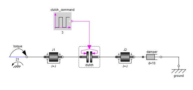
If this were a friction clutch, the behavior of the clutch would depend strongly on the inertia of the shafts on either side as well as the amount of torque driving the J1 shaft. In order to get the clutch to engage smoothly over a specified time, we would have to create a complex control system that was tuned to the characteristic of the system (amount of torque being transmitted through the clutch, amount of inertia on either side of the clutch, etc).

But, since this is a kinematic clutch with the response of the clutch being prescribed, we can ensure the proper function of the clutch independent of these other factors. To demonstrate this, we start with a baseline system and specify an engagement time of 800 milliseconds. If we simulate this baseline system, we can see the engagement process in the following figure:

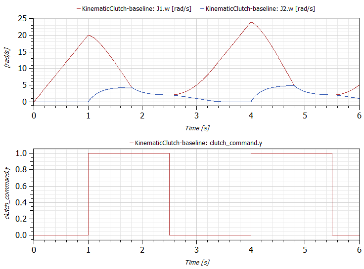
Note the engagement time is 800 milliseconds, as expected. We see the convergence of the red and blue lines (representing the speeds of the two shafts) exactly as we prescribed it. Now, to demonstrate that our kinematic clutches response is completely independent of the other design characteristics of the system, we increase the applied torque by 50% and we decrease the inertia of the left shaft by 25%. In that case, we get the responses shown by the green and violet lines in the following figure:

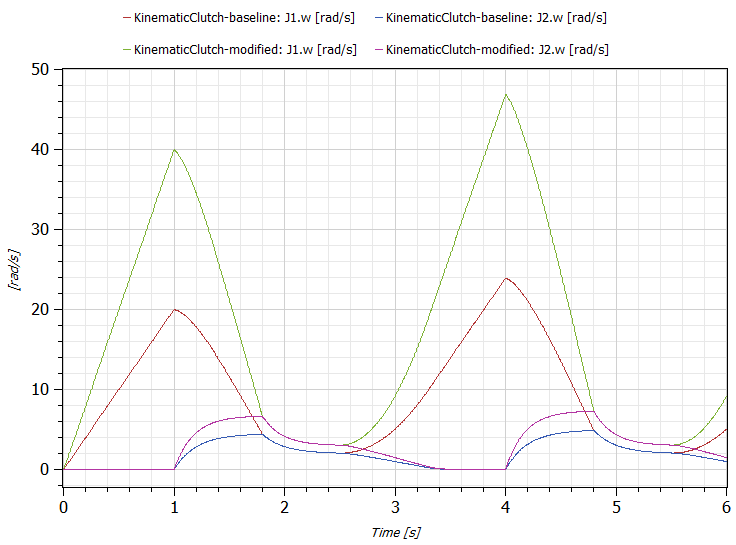
Note that we have retained the original response in this plot (the red and blue lines) so we can see that while the physical responses are different while the clutches are disengaged (the left shaft accelerates much more in our modified system due to the greater torque and less inertia), the timing of the engagement is identical. In other words, our clutches functional behavior is identical in both cases.

Now it may seem rather trivial to enforce the speed response of the clutch. But remember we are actually imposing a kinematic constraint on the rest of the system. Since these are acausal models, we are including equations for conservation of angular momentum throughout our system. This means that the reaction torques associated with these kinematic constraints must be computed. Figure 5 shows a comparison between the reaction torques imposed by our kinematic clutch model between our baseline and modified models.

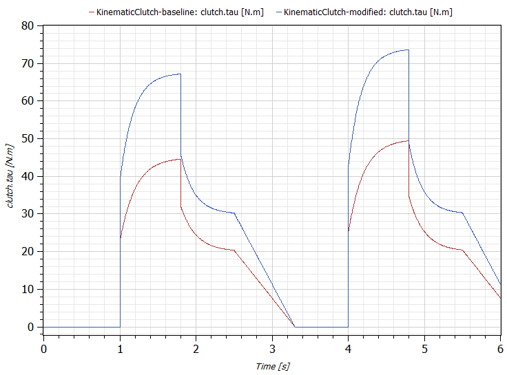
Computing these reaction torques is not straightforward and in order to do so a system of implicit equations must be solved.

When performing high level system analyses, this kind of reaction torque information can be used to cascade requirements to the lower level subsystems and components. For example, we see in this case that for one design we expect a peak torque for the clutch to be only 50 N.m while in the other case it is 74 N.m.

Conclusion

The purpose of the kinematic clutch model is to allow you to temporarily side-step the challenges associated with designing a production quality control system for clutch engagement when you are trying to analyze "the big picture" of system level performance. A common context for this would be drive cycle modeling for different transmission concepts. In these cases, we are interested in the potential of the concept and don't want to get overly bogged down (at this point) in the details of how to actually achieve the desired functionality. By making the assumption that the clutches will function as expected, you can focus on high level system design during this upfront process.

Then, when you have finished this high level design work and validated your concept, you can move down the system engineering "V" and begin to look at subsystem design. In the process, you can cascade your high level requirements (e.g. necessary torque capacity on your clutches, desired engagement times, etc) down to your subsystems. At that point (and using some nice features in Modelica that we didn't talk about here), you can refine your subsystem models by replacing your functional clutch models with predictive models. This will bring all of the subsystem design parameters for the physical design (geometry, materials, hydraulics) as well as the design of the controller itself into the picture.