Redux

In a previous post, I talked about how to take models expressed as a system of equations and turn them into a component based approach. Unfortunately, I think the domain I used in that case limited how much depth I could go into (partly due to the complexity of the underlying models and partly due to the fact that I don't have much domain expertise in that area).

I wasn't really very happy with my previous attempt. So I decided to try again. This time, I'm going to use a simpler system and try and explore it more completely. As with some of my previous posts, the models I'm discussing are available on GitHub under a Creative Commons Attribution 3.0 Unported License.

Lotka-Volterra

Base Equations

The basis for this post will be the Lotka-Volterra equation. The basic form of the Lotka-Volterra equation is:

\begin{aligned} \dot{x} & = x ( \alpha - \beta y) \\ \dot{y} & = -y ( \gamma - \delta x) \end{aligned}

For those unfamiliar with these equations, they are meant to model the relationship between two populations of animals. One population, x, represents the "prey" in this relationship and the other population, y, represents the "predators". For this reason, the Lotka-Volterra equation is sometimes referred to as a "predator-prey" model.

The left hand terms clearly represent the fluctuations in each population. Right hand terms represent reproduction, starvation and predation. We will be discussing these effects in detail shortly.

If we wanted to simply convert this to Modelica, it is quite straightforward:

model ClassicModel "This is the typical equation-oriented model"
  parameter Real alpha=0.1;
  parameter Real beta=0.02;
  parameter Real gamma=0.4;
  parameter Real delta=0.02;
protected
  Real x(start=10);
  Real y(start=10);
equation
  der(x) = x*(alpha-beta*y);
  der(y) = -y*(gamma-delta*x);
end ClassicModel;

For the most part, this model maps directly to the equations. There are two exceptions worth mentioning at this point. The first is the assignment of actual values to alpha, beta, gamma and delta. In order to simulate the model, I need to provide some actual values for these. The other addition compared to the basic equations is the addition of the start=10 modification for the variables x and y. We'll see the need for those shortly.

Running the "Classic" model

If we run the simulation, we get results like those shown below.

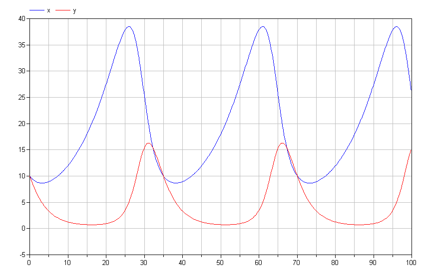
Note the cyclical nature of x and y. This is typical of the Lotka-Volterra model. If we plot y vs. x, we get the following limit cycle.

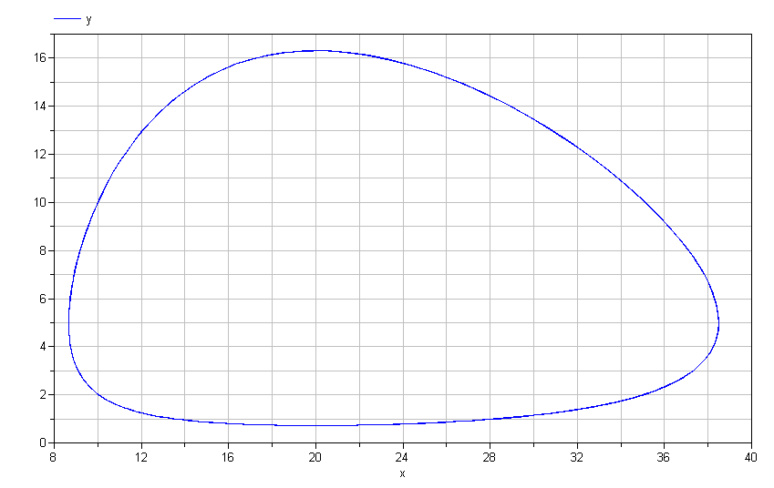
Mathematically speaking, this limit cycle will continue forever. There is no "damping" present in these equations. Does this mean that no matter what initial conditions you choose, you will invariably have such dynamics?

No.

There are initial conditions that are stable. For these conditions, the rate at which the prey are eaten exactly balances the rate at which they are born. Furthermore, the rate at which the predators die from starvation is equal to the rate at which new predators are born (supported by the consumption of the prey).

You might wonder how, for a given set of values for alpha, beta, gamma and delta, we might determine what those initial conditions are. This is where Modelica's rich initialization capabilities come in very handy. In this case, we can create a quiescent version that extends from the classic model and adds two equations that are applied to solve (only) for the initial conditions:

model QuiescentClassicalModel "Adding quiescent initial conditions"
  extends ClassicModel;
initial equation
  der(x) = 0;
  der(y) = 0;
end QuiescentClassicalModel;

The extends keyword in Modelica is very important. It allows you to inherit (i.e., automatically insert) the contents of another model into the current model. In this way, we can reuse code between different models without having to repeat it all the time. So in this case, we want to reuse the dynamic equations from ClassicModel but add two additional equations to solve for the initial values of x and y.

This is where that start attribute comes into play...

Give me a hint

The start attribute is complicated because its "meaning" depends on a couple of factors. I'll discuss two important cases.

In the ClassicModel, there are no explicit initial conditions for x and y. If there were, they would look something like this:

initial equation
  x = 5.0;
  y = 7.3;

But since there aren't any initial conditions, what should a tool use for initial conditions? In this case, the tools look for hints about what to do and the start attribute is that hint. Most tools will see that x and y have no initial conditions and will choose to use whatever value the start attribute has as initial conditions.

In the QuiescentClassicalModel, we have explicit initial conditions (exactly enough). For initialization purposes, you can consider \(\dot{x}\), \(x\), \(\dot{y}\) and \(y\) to all be completely independent variables. We then combine the initial equations with the dynamic equations to arrive at:

\begin{aligned} \dot{x} & = x ( \alpha - \beta y) \\ \dot{y} & = -y ( \gamma - \delta x) \\ \dot{x} & = 0 \\ \dot{y} & = 0 \end{aligned}

Obviously, we can easily eliminate the variables \(\dot{x}\) and \(\dot{y}\) and we are left with a simple non-linear system to solve for the initial values for \(x\) and \(y\):

\begin{aligned} 0 & = x ( \alpha - \beta y) \\ 0 & = -y ( \gamma - \delta x) \end{aligned}

Note I said "non-linear". When solving any non-linear system you have the potential for multiple solutions¹. If numerical methods are used to solve such a system, an initial guess for the variables involved is used to help guide the solver toward a particular solution among the many that are possible. Once again, the start attribute provides the "hint" that specifies what values should be used (in this case by the non-linear solver, not the integrator).

Get to the Component Models!

So far, we have simply introduced the equation oriented version of the system we wish to explore. Let's quickly get started with component models.

Connectors

When building libraries of components, the very first thing that you need to do is define the connector(s) you intend to use. The connector defines the information that is to be shared between components. In our case, we are interested in the "flow" of things (animals) so we will use a connector like this²:

connector Population "A connector for a population of animals"
  Real population "Animal population";
  flow Real rate "'Flow' of animals through this connector";
end Population;

This says that our components will share information about the population at a given point and about the change in the population due to a particular interaction between components. Concrete examples will follow shortly.

Regional Population

The left hand terms in the Lotka-Volterra equation represent the change in a given animal population within some region. A Modelica model that performs the same bookkeeping for the population in a given region would look like this:

model RegionalPopulation "A localized population of animals"
  Population pop;
  parameter Boolean steady_state;
  parameter Real initial_population;
protected
  Real population(start=10) = pop.population;
initial equation
  if steady_state then
    der(population) = 0;
  else
    population = initial_population;
  end if;
equation
  der(population) = pop.rate;
  assert(population>=0, "Population went negative!");
end RegionalPopulation;

This may look complicated at first, but it isn't really. Most of the complexity comes from the parameter called steady_state which indicates whether we want to specify an initial population value or if we would like to use an initial population that will lead to a quiescent state. The population variable represents the population in this region. The equations relate the local population to the population specified on the connector and the "flow" of animals coming or going via the connector.

Interactions

Now we need to implement the various interactions on the right hand side of the Lotka-Volterra equations. We will start with birth which is assumed to be proportional to the size of the population (hence more breeding pairs). The constant of proportionality is \(\alpha\) and we might define the reproduction model as follows:

model Reproduction "Model of reproduction"
  Population pop;
  parameter Real alpha "Birth rate";
equation
  pop.rate = -alpha*pop.population;
end Reproduction;

We might write the model this way, but I chose not to. The reason is that Modelica follows a convention that "flow" into a component is always positive³. This convention actually makes the population model intuitive, i.e.,

equation
  der(population) = pop.rate;

However, for the various interactions we'd like to model, it makes it a little heard to read. When you see:

equation
  pop.rate = -alpha*pop.population;

you have to pause for a moment to really consider if this is correct (it is, BTW). So I created the following "base classes" to introduce a more intuitive terminology. The first, SinkOrSource, is for interactions like reproduction or starvation that simply add or remove animals. The other, Interaction, is for interactions like migration or predation that affect two different populations. The definitions of these two base class models are as follows:

partial model SinkOrSource "Model for population dynamics that are either sinks or sources"
  Population pop;
protected
  Real growth "Growth in the population (if positive)";
  Real decline "Decline in the population (if positive)";
equation
  decline = -growth;
  pop.rate = decline;
end SinkOrSource;

partial model Interaction "Modeling interaction between two populations"
  Population pop_a;
  Population pop_b;
protected
  Real a_growth "Growth in population a that results from this interaction";
  Real a_decline "Decline in population a that results from this interaction";
  Real b_growth "Growth in population b that results from this interaction";
  Real b_decline "Decline in population b that results from this interaction";
equation
  a_decline = -a_growth;
  pop_a.rate = a_decline;
  b_decline = -b_growth;
  pop_b.rate = b_decline;
end Interaction;

These definitions are useful because a model that extends from them simply needs to provide an equation for either the growth or decline associated with each population (connector). This, in turn, will make the intent of the model much clearer.

Since these models are not complete models, but simply meant to be a starting point for other models (defining common elements like connectors and variables), they are marked partial to make it clear that they themselves cannot be instantiated.

By extending from the SinkOrSource model, we can make a more intuitive birth model:

model Reproduction "Model of reproduction"
  extends SinkOrSource;
  parameter Real alpha "Birth rate";
equation
  growth = alpha*pop.population;
end Reproduction;

as well as an easy to understand starvation model:

model Starvation "Starvation model"
  extends SinkOrSource;
  parameter Real gamma "Starvation coefficient";
equation
  // Rate of starvation is proportional to population
  decline = gamma*pop.population;
end Starvation;

The key point in these models is that the user has to provide an equation for either the decline or the growth variable and the SinkOrSource model will make sure that the proper equation is applied to the flow variable on the connector and make the intent of the equations a bit clearer.

In order to complete the interactions in a classic Lotka-Volterra equation, the only thing left to model is the predation. Extending the partial Interaction model, our predation model looks something like this:

model Predation "Model of predation"
  extends Interaction;
  parameter Real beta "Prey consumed";
  parameter Real delta "Predators fed";
equation
  b_growth = delta*pop_a.population*pop_b.population;
  a_decline = beta*pop_a.population*pop_b.population;
end Predation;

As with reproduction, "you need two to tango" so this the equation has a form very much like equations that arise from the "Law of Mass Action". Unlike the reproduction model, one of the two parties involved declines as a result of the interaction. This is clearly reflected through the use of the b_growth and a_decline variables.

Kicking the Tires

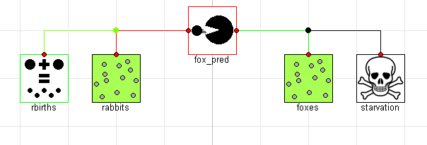
Now that we have all the interactions, we can put everything together. There are two obvious benefits to the component oriented approach at this point. The first is that we write the equations for each of the various effects once and capture them in a component model which we will have no need to modify. The other advantage is that we can now compose our systems graphically⁴. By dragging and dropping down two populations (rabbits and foxes) as well as instances of the reproduction, predation and starvation models we can very easily compose an equivalent component-oriented version of the class Lotka-Volterra equation:

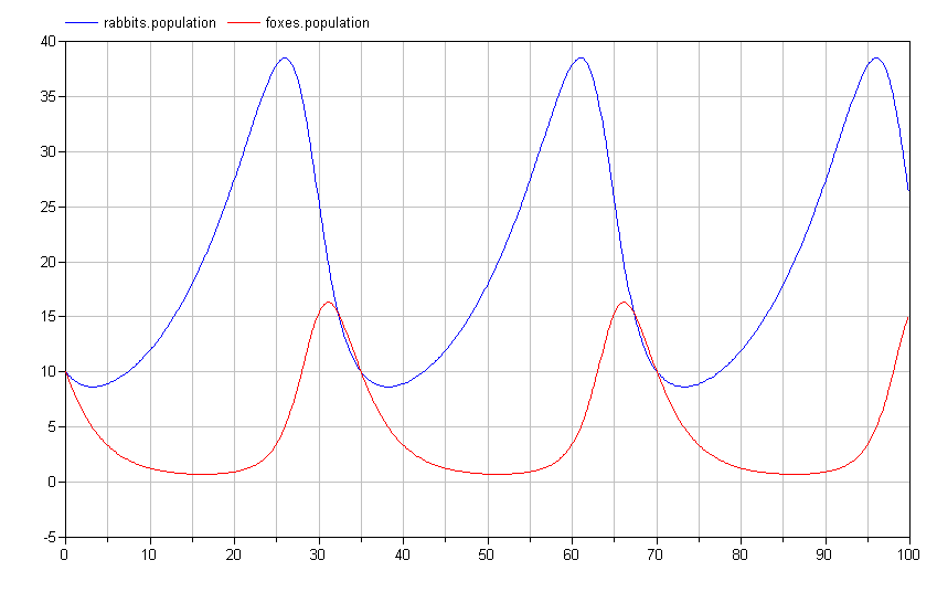
If we simulate this model, we see that the results are identical (although the names of the signals are now different and arguably more informative):

The actual Modelica code for this system would be:

model ComponentOriented "A component-oriented version of the Lotka-Volterra system"
  RegionalPopulation rabbits(initial_population=10, steady_state=steady_state);
  RegionalPopulation foxes(initial_population=10, steady_state=steady_state);
  Starvation starvation(gamma=0.4);
  Reproduction rbirths(alpha=0.1);
  Predation fox_pred(beta=0.02, delta=0.02);
  parameter Boolean steady_state = false;
equation
  connect(starvation.pop, foxes.pop);
  connect(rbirths.pop, rabbits.pop);
  connect(fox_pred.pop_b, foxes.pop);
  connect(fox_pred.pop_a, rabbits.pop);
end ComponentOriented;

For those not familiar with Modelica, the lines that connect the different models (called connections) add special equations to the overall system. For a variable with the flow qualifier, it applies a generalized version of Kirchhoff's Current Law. This is essentially a conservation principles that ensures that anything (animals in this case) that leaves one component ultimately ends up in another⁵. For the other variables on the connector, equations are added to make sure that the variables have the same value across all the connected connectors.

At this point, you might be thinking "With the component-oriented approach, we seem to have done a lot more work for the same effect." This is true, but it was an up-front investment to make subsequent modeling much more scalable.

What I find really exciting about this approach is how easily it is to create new configurations of these different effects and how quickly I can explore those "designs". I often tell people that by building up such component libraries, you are making your very own Erector Set for the particular domain you are interested in (e.g., population dynamics).

Rabbits and Foxes and Wolves, Oh My!

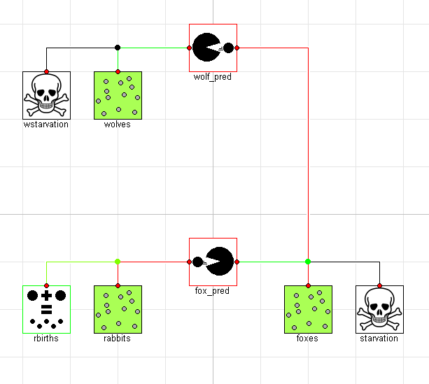
To demonstrate this, let's imagine we wanted to add a new predator to the mix. We could easily do this as follows:

model ThreeTier "The hunter becomes the hunted"
  extends ComponentOriented;
  RegionalPopulation wolves(initial_population=10, steady_state=steady_state);
  Predation wolf_pred(beta=0.04, delta=0.08);
  Starvation wstarvation(gamma=0.4);
equation
  connect(wstarvation.pop, wolves.pop);
  connect(wolves.pop, wolf_pred.pop_b);
  connect(wolf_pred.pop_a, foxes.pop);
end ThreeTier;

Graphically, this system would look like this:

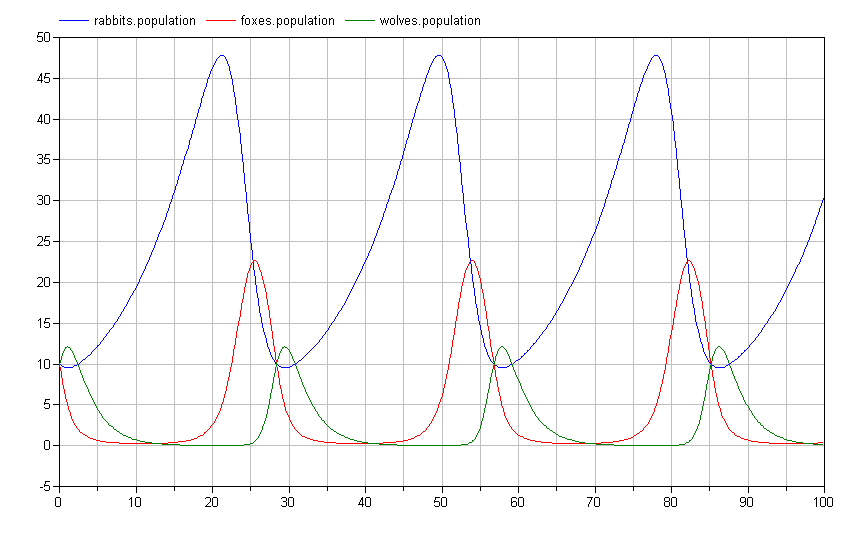
If we simulate this system, we again see a limit cycle where the populations repeat their trajectories over the period of the limit cycle:

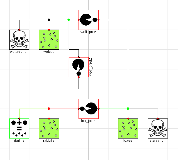
Of course, it is impossible to imagine with a bunch of rabbits running around that wolves would only eat the foxes. To address this, we add an additional predation connection between the wolves and the rabbits as follows:

model ThreeTierOmnivores "Wolves will eat anything"
  extends ThreeTier;
  Predation wolf_pred2(beta=0.02, delta=0.01);
equation
  connect(wolf_pred2.pop_b, wolves.pop);
  connect(wolf_pred2.pop_a, rabbits.pop);
end ThreeTierOmnivores;

Graphically, the model would then look like this:

Interestingly, this causes an important shift in the ecosystem. By having two predators feeding on the prey at the bottom of the food chain, we see much more dramatic swings in the population:

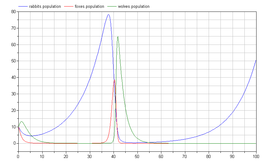
Note how the rabbit population soars before the wolf and fox populations have a chance to rebound? Perhaps we shouldn't give those rabbits such a free ride. Let's introduce a disease model to deal with over-population:

model Disease "Non-linear disease model"
  extends SinkOrSource;
  parameter Real zeta "Disease coefficient";
equation 
  // Rate of starvation is proportional to population
  decline = zeta*pop.population*pop.population;
end Disease;

Like the Reproduction and Starvation models, this extends from the SinkOrSource model. It resembles the Reproduction model with two key differences. First, it is obviously moving in the other direction (killing off the population in question). Second, it is not just proportional to the population, but proportional to the square of the population⁶.

Adding this Disease model to our system is as simple as:

model ThreeTierWithDisease "Add disease for rabbits"
  extends ThreeTierOmnivores;
  Disease rdisease(zeta=1e-3);
equation
  connect(rdisease.pop, rabbits.pop);
end ThreeTierWithDisease;

Down the Rabbit Hole

Just when you thought we couldn't dig into this subject any deeper, let's consider some additional dynamics that could make the system more interesting. Our system so far is concerned with the RegionalPopulation for each species. But what if we wanted to apply all of these dynamics in multiple regions?

The first thing we would need to do would be to take our system and turn it into a model that can interact with external influences. To do this, we can extend the ThreeTierWithDisease model and add some connectors to allow it to connect to those external influences as follows:

model RegionEcosystem "Include all the dynamics but for a single region"
  extends ThreeTierWithDisease;
  Population w "Interaction with wolves";
  Population f "Interaction with foxes";
  Population r "Interaction with rabbits";
equation
  connect(wolves.pop, w);
  connect(foxes.pop, f);
  connect(rabbits.pop, r);
end RegionEcosystem;

Now we have all the dynamics of our ThreeTierWithDisease model wrapped up in something that we can instantiate multiple times. But what makes this more interesting is if we have interactions between each region. For this, we add a migration model as follows:

model Migration "Simple proportional migration model"
  extends Interaction;
  parameter Boolean initially=false "Allow migration at initialization?";
  parameter Real mu "migration constant";
protected
  Real migration_rate "Departure rate (immediate) from region a to region b";
equation
  if initial() and not initially then
    migration_rate = 0;
 else
    migration_rate = mu*(pop_a.population-pop_b.population);
  end if;
  a_decline = migration_rate;
  b_growth = migration_rate;
end Migration;

This model causes the population for a given species to move from a more populated region to a less populated one. This is an overly simplistic model. A real model would probably consider factors like availability of food on both ends, distance between regions, delay in moving from one region to another, etc.

Now, let's creates a model that includes four different regions and provides migration patterns for the fox and wolf populations across various regions. Graphically, the model looks like this:

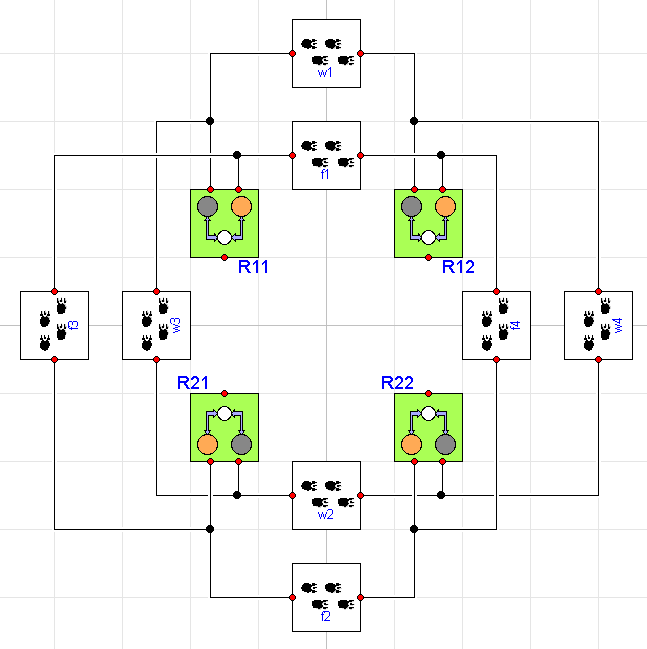
where each region includes the ThreeTierWithDisease ecosystem we showed earlier. Now we can start to understand why this approach is so much more scalable. We've only added two additional interactions to get to this point (Disease and Migration). Using this handful of component models, we've created a system with 12 distinct populations (differential equations) and 32 different effects (resulting in 54 right hand side terms) and we did it without having to write or change a single equation (beyond those in the component models).

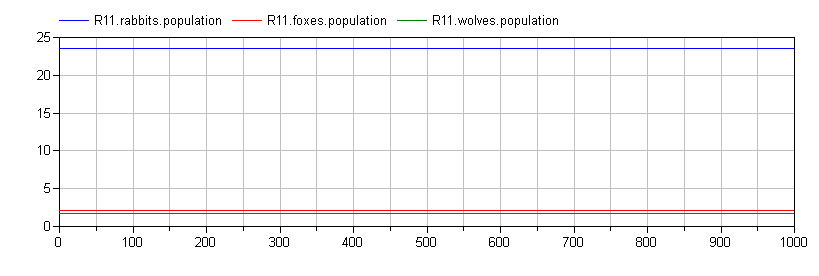
To see the effects of migration, let us configure our model such that one region is in a quiescent state to begin with (remember our steady_state parameter?) but the others are not. Without migration, the quiescent region would have no population dynamics. But because of migration, the other regions destabilize the quiescent population.

The following figures show the effect of fox migration on the dynamics in the (initially) quiescent region for increasing levels of fox migration (starting with none):

These are the kinds of results that I find fascinating. Note how the qualitative dynamics of the system change significant simply by introducing fox migration between the regions.

Conclusion

Given the length of this post, I'm impressed you got this far.

Hopefully, this post demonstrates how much better the component-oriented approach scales. Not only does it allow you to create a library of reusable component models that capture the various effects of interest, it helps avoid the manual (and therefore tedious, time-consuming and error prone) process of writing down all the bookkeeping equations that track how animals appear or disappear in the various populations and, finally, it enables a graphical approach to building complex system models.

I've left out lots of interesting possibilities. For example, I didn't include models for effects like Mutualism or Parasitism.

Although I've used a non-engineering (but hopefully intuitive and easy to understand) domain, all of what I've discussed here is used in the building models of engineering systems. Instead of tracking the flow of rabbits, we track the flow of conserved quantities like mass, momentum, charge, elements, energy and so on.

There are some additional advanced topics that I originally planned to include but this post is already too long so I left them out. However, the examples are present in the source code on GitHub.