Today's Topic

If you are not familiar with Fourier Analysis, the purpose of the analysis is to represent a function as the weighted sum of a collection of trigonometric functions (sines and cosines). This, in turn, allows us to extract the spectral properties of the function.

In this case, we are going to explicitly construct the Fourier series of an input signal. This will not only give us the coefficients for each sine and cosine term in the range of frequencies we are interested in, but it will also give us the phase and magnitude of those frequencies as well.

Mathematically Speaking

Before diving into the Modelica code, let's be clear about what is really going on here mathematically. Assume we have some input signal, \(u\), that we are interested in analyzing. Further assume that the frequencies we are interested in are the first \(n\) harmonics of a base frequency, \(F_0\) (i.e., \(F_0\), \(2 F_0\), \(3 F_0\), ..., \(n F_0\)).

What we wish to solve for are the coefficients \(a_i\) and \(b_i\) such that:

\[u = \frac{a_0}{2} + \sum_{i=1}^{n} \left[ a_i cos(2 \pi i F_0 t) + b_i sin(2 \pi i F_0 t) \right] \]

where \(F_0\) is in Hertz. So the question is, how do we compute \(a_i\) and \(b_i\)?

Fortunately, Jean-Baptiste Joseph Fourier already worked that out for us. It turns out to be relatively simple. We integrate over the period of our base frequency as follows:

\[a_i = 2 \int_{t=0}^{\frac{1}{F_0}} u\ cos(2 \pi i F_0 t) \]

and

\[b_i = 2 \int_{t=0}^{\frac{1}{F_0}} u\ sin(2 \pi i F_0 t) \]

If we manage to work out \(a_i\) and \(b_i\), then we can compute the phase, \(\phi_i\), and magnitude, \(m_i\) using the following relationships:

\[\phi_i = tan^{-1}(b_i/a_i)\]

\[m_i = \sqrt{a_i^2+b_i^2} \]

Fourier Analysis Model

When we want to apply all this math to the behavior of a model, all we need to do is build a simple signal processing block that performs these integrals and applies these relationships.

Let's take this bit by bit. First, what is the "public interface" of the component (the parts the user has to know about)? It should include a parameter for the fundamental frequency, a way to feed a signal in for analysis and way to extract the various analysis results as output. In other words:

parameter Modelica.SIunits.Frequency F0 "Base frequency for analysis";
parameter Integer n "Number of harmonics";
Modelica.Blocks.Interfaces.RealInput u "Input signal";
Modelica.Blocks.Interfaces.RealOutput a0 "Signal bias";
Modelica.Blocks.Interfaces.RealOutput a[n] "Fourier coefficients for cosine terms";
Modelica.Blocks.Interfaces.RealOutput b[n] "Fourier coefficients for sine terms";
Modelica.Blocks.Interfaces.RealOutput mag[n] "Magnitude for each frequency";
Modelica.Blocks.Interfaces.RealOutput phase[n] "Phase for each frequency";

Internal to the model, there are a number of things we would like to compute. So we'll create a protected section for those:

protected
  parameter Modelica.SIunits.Time dt = 1.0/F0 "Period at base frequency";
  Real s[n] = {sin(2*pi*F0*i*time) for i in 1:n} "Sine waves at various frequencies";
  Real c[n] = {cos(2*pi*F0*i*time) for i in 1:n} "Cosine waves at various frequencies";
  Real a0i "Integral of bias term";
  Real ai[n] "Integral of cosine terms";
  Real bi[n] "Integral of sine terms";
  Real f "Reconstructed function";

where s is a vector of the sine functions at each of the various frequencies we are interested in, c is a vector of cosine functions at those same frequencies. We will use a0i, ai and bi to hold the values of various integrals. Finally, f will compute the value of our input signal approximated as a Fourier series (delayed by one period of our fundamental frequency.

At the start of our simulation, we initialize all our integral terms to zero:

initial equation
  a0i = 0;
  ai = zeros(n);
  bi = zeros(n);

We also have the following continuous equations in our models to compute the various integrals, the reconstructed function, phase and magnitude:

equation
  der(a0i) = 2*u;
  der(ai) = 2*u*c;
  der(bi) = 2*u*s;
  f = a0/2+a*c+b*s;
  mag = {sqrt(a[i]^2+b[i]^2) for i in 1:n};
  phase = {atan2(b[i], a[i]) for i in 1:n};

These equations demonstrate some of the interesting vector related functions in Modelica. For example, * is used as both multiplication (scalar times vector) and as an inner product (between vectors) in expressions like 2*u*c. We also use the array comprehensions feature to compute the magnitude and phase. This allows us to write down an expression for the \(i^{th}\) element of a vector.

The only complicated part of the model is what we do at the end of each period of our fundamental frequency. This is represented in the following when clause:

equation
  // ...
  when sample(0,dt) then
    a0 = pre(a0i);
    a = pre(ai);
    b = pre(bi);
    reinit(a0i, 0);
    for i in 1:n loop
      reinit(ai[i], 0);
      reinit(bi[i], 0);
    end for;
  end when;

At the end of each period of our fundamental frequency, we extract the current value of our integral variables (a0i, ai and bi) and assign their values to the coefficients in the series. Then, we use the reinit function to reinitialize those integrals so they start from zero again.

Putting this all together, our model looks like this:

within Sensors.SignalProcessing;
model FourierAnalysis "Compute Fourier coefficients of an input signal"
  parameter Modelica.SIunits.Frequency F0 "Base frequency for analysis";
  parameter Integer n "Number of harmonics";
  Modelica.Blocks.Interfaces.RealInput u "Input signal";
  Modelica.Blocks.Interfaces.RealOutput a0 "Signal bias";
  Modelica.Blocks.Interfaces.RealOutput a[n] "Fourier coefficients for cosine terms";
  Modelica.Blocks.Interfaces.RealOutput b[n] "Fourier coefficients for sine terms";
  Modelica.Blocks.Interfaces.RealOutput mag[n] "Magnitude for each frequency";
  Modelica.Blocks.Interfaces.RealOutput phase[n] "Phase for each frequency";
protected
  import Modelica.Constants.pi;
  import Modelica.Math.atan2;
  parameter Modelica.SIunits.Time dt = 1.0/F0 "Period at base frequency";
  Real s[n] = {sin(2*pi*F0*i*time) for i in 1:n} "Sine waves at various frequencies";
  Real c[n] = {cos(2*pi*F0*i*time) for i in 1:n} "Cosine waves at various frequencies";
  Real a0i "Integral of bias term";
  Real ai[n] "Integral of cosine terms";
  Real bi[n] "Integral of sine terms";
  Real f "Reconstructed function";
initial equation
  a0i = 0;
  ai = zeros(n);
  bi = zeros(n);
equation
  der(a0i) = 2*u;
  der(ai) = 2*u*c;
  der(bi) = 2*u*s;
  f = a0/2+a*c+b*s;
  mag = {sqrt(a[i]^2+b[i]^2) for i in 1:n};
  phase = {atan2(b[i], a[i]) for i in 1:n};
  when sample(0,dt) then
    a0 = pre(a0i);
    a = pre(ai);
    b = pre(bi);
    reinit(a0i, 0);
    for i in 1:n loop
      reinit(ai[i], 0);
      reinit(bi[i], 0);
    end for;
  end when;
end FourierAnalysis;

I've included this FourierAnalysis block in my open source Sensors package on GitHub.

Testing

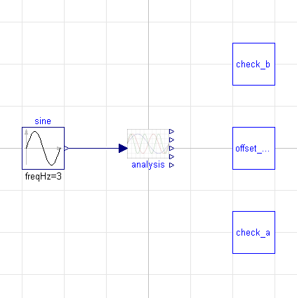
Now, I would never really undertake building a model like this without testing it. Let's first consider a case where we have only a single sine wave as an input. In this case, let's make the frequency of that sine wave three times that of our fundamental frequency. In diagram form, our test looks like this:

A simple way to determine whether the model is correct is to do a visual comparison between the input signal and the reconstructed function, f, contained within the FourierAnalysis block. This works particularly well if each period of the input signal is identical. In the following figure, we can see a comparison between the input and reconstructed functions. We see clearly that they are identical.

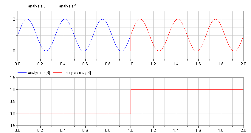
In the figure above, we also see the values for b[3] and mag[3] which should both match the magnitude of the input signal, u, as expected.

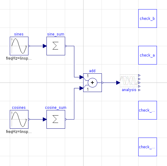
Another test we can do is to add together many different sine and cosine waves of different magnitudes into a single waveform and then see of our FourierAnalysis block can extract them back out. That is the approach behind our second test:

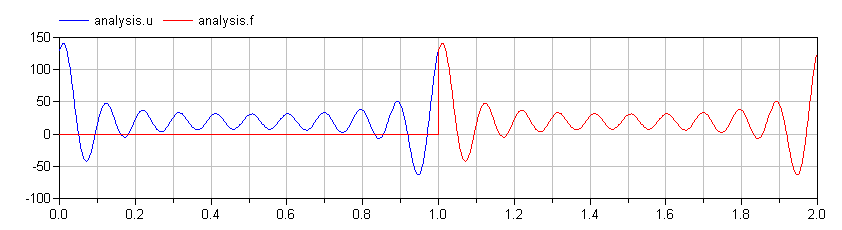
Again, since this function repeats itself with every period, we can compare the input function to the reconstructed function for a quick visual confirmation:

Conclusion

This is an example of how a useful analytical technique like Fourier analysis can be implemented in Modelica. Such a block can then be used to perform on-the-fly analysis while simulating a Modelica model.

As always, the source code from these examples can be found on GitHub. The code is distributed under a Creative Commons license so you can feel free to use the code in your own projects.