In theory, there is no difference between theory and practice. In practice, there is.
-- Yogi Berra

Welcome to the Real World

A while back, I was talking with a couple of professor friends of mine once about control systems and the big difference between the mathematical aspects of control and the real-world aspects. They were telling me how their institution starts with a bunch of classes on control theory and then the students have to do a practical controls lab using Lego Mindstorms.

I was joking they should hang a sign over the lab that said "Welcome to the Real World". If you haven't had to cross this particular chasm, the issue here is that there is hardly anything mathematical about embedded controls. All the elegance of the math is demolished by limitations in CPU power, memory, bandwidth, signal resolution, noise, etc.

Which brings me to my topic for this post...

Sensor Modeling

There is a lot you can say about sensor (and actuator modeling). Sensors and actuators are subject to far too many limitations to discuss here. I'm only going to really show two examples and hopefully you'll get the idea. The complete source for these examples is, once again, hosted on GitHub under a Creative Commons Attribution 3.0 Unported License

Talking about how to model real world sensors and the artifacts that result is a great chance to discuss how to model the interactions between continuous systems and discrete systems. For the purposes of this post, I'm going to talk about angular velocity sensors. I'll cover just two (of the many) ways you can approximate speed in an angular velocity sensor.

Both of these methods assume that we will receive a certain number of "pulses" per revolution¹. This is typical for rotary speed sensors. We'll use these pulses in two different ways. The first approach for estimating speed will involve counting how many pulses occur in a specified time interval. The other approach will involve measuring the time between pulses. As we will see, each of these approaches has their own specific advantages and disadvantages.

Before we get started

All the sensor models I will present will extend from this base class:

within Sensors.Interfaces;
partial model RotarySpeedSensor "Base class for all rotary speed sensor models"
  extends Modelica.Mechanics.Rotational.Interfaces.PartialAbsoluteSensor;
  Modelica.Blocks.Interfaces.RealOutput w_estimate;
protected
  Modelica.SIunits.Angle angle = flange.phi;
end RotarySpeedSensor;

What this base class does is it pulls in the nice graphics of the PartialAbsoluteSensor base class as well as the rotational flange connector. I've added a protected variable which is simply an alias for the angle of the shaft we are interested in. I've also added an output signal for us to send our speed estimate to.

By creating such an interface, I can create an architecture for all of my tests that looks like this:

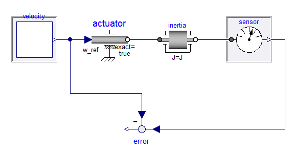
In source code form, this looks like:

within Sensors.Tests;
partial model SensorTest "Base class for sensor testing"
  replaceable Modelica.Blocks.Interfaces.SO velocity;
  replaceable Sensors.Interfaces.RotarySpeedSensor sensor;
  Modelica.Mechanics.Rotational.Components.Inertia inertia(J=1);
  Modelica.Mechanics.Rotational.Sources.Speed actuator(exact=true);
  Modelica.Blocks.Math.Feedback error;
equation
  connect(velocity.y, actuator.w_ref);
  connect(actuator.flange, inertia.flange_a);
  connect(sensor.flange, inertia.flange_b);
  connect(velocity.y, error.u2);
  connect(sensor.w_estimate, error.u1);
end SensorTest;

Counting Method

Now that I have my RotarySpeedSensor model in place, I'm ready to build my "tooth counting" sensor model. The model I created looks like this:

within Sensors.RotarySpeed;
model ToothCounter "Estimate speed by counting 'pip' signals"
  extends Sensors.Interfaces.RotarySpeedSensor;
  parameter Integer teeth "Number of teeth";
  parameter Modelica.SIunits.Time sample_rate;
protected
  parameter Modelica.SIunits.Angle tooth_angle = Modelica.Constants.pi*2/teeth;
  Modelica.SIunits.Angle next_angle;
  Integer count(start=0);
algorithm
  when initial() then
    next_angle := angle+tooth_angle-mod(angle,tooth_angle);
    w_estimate := 0;
  end when;
  when {angle>next_angle, angle<next_angle-tooth_angle,
        angle<next_angle-2*tooth_angle} then
    count := pre(count)+1;
    next_angle := angle+tooth_angle;
  end when;
  when sample(sample_rate,sample_rate) then
    w_estimate := (count-0.5)*tooth_angle/sample_rate;
    count := 0;
  end when;
end ToothCounter;

The teeth parameter represents how many teeth there are on the wheel (i.e., how many pulses per revolution we can expect). The sample_rate parameter indicates how often we will check our tally of pulses. These are both public parameters. There is one protected parameter, tooth_angle. This is the angle between each pulse.

You might ask why is this a parameter since most people think a parameter is something that the user has to enter. In Modelica, a parameter is something that won't change during the simulation. If the parameter doesn't have a binding equation, then the user needs to provide it. But in the case of tooth_angle, there is a binding equation so the parameter will be computed (from other parameters). You might also wonder why this is in a protected section. A protected section is used to hide implementation details. I tend to put everything the user doesn't need to know about (or things that might confuse the user) in a protected section.

But the meat of this model is in the variables next_angle and count. Let's start with count since it just represents the number of times (in the current sample interval) that a pulse has been detected. This counting process is expressed later in the model by the following when clause:

when {angle>next_angle, angle<next_angle-tooth_angle,
      angle<next_angle-2*tooth_angle} then
  count := pre(count)+1;
  next_angle := angle+tooth_angle;
end when;

The when clause is triggered if any of the three conditions inside the {...} becomes true. These three conditions represent the three nearby teeth.

Why three? If you are between any two teeth, isn't it sufficient to just detect either of those? Yes, if you are between two teeth. But it is also possible to be on a tooth (e.g., at the start of the simulation). So this covers that corner case.

But regardless which tooth triggers the pulse, we handle it the same. We determine the angle of the next tooth (in the positive angular direction) and we count the tooth we just sensed.

So where does the speed come from? It comes from this when clause:

when sample(sample_rate,sample_rate) then
  w_estimate := (count-0.5)*tooth_angle/sample_rate;
  count := 0;
end when;

This is the when clause that counts the number of pulses at the end of every sample interval and makes a speed estimation based on that.

If we extend from our SensorTest model, add this sensor and drive it with an exponential sine wave speed profile, i.e.,

within Sensors.Tests.ToothCounter;
model TestToothCounter
  extends SensorTest(redeclare Modelica.Blocks.Sources.ExpSine velocity(
      amplitude=100, freqHz=5,
      offset=50, damping=1),
    redeclare replaceable Sensors.RotarySpeed.ToothCounter sensor(
      teeth=72, sample_rate=0.01));
  XogenyTest.AssertInitial iw(expected=0, actual=sensor.w_estimate);
end TestToothCounter;

...we get a speed estimation that looks like this:

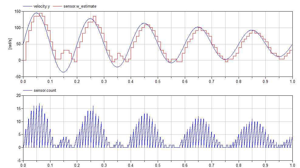
I've also included a plot of the count variable so you can see how many pulses occur in each interval. Note, if you only measure pulses, you cannot determine the direction of motion. You can see that clearly in the speed estimate.

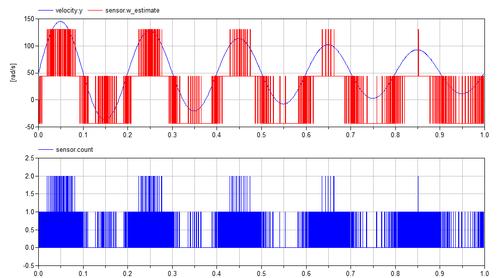
An interesting thing about such sensors is that high sampling rates can give you less accuracy, not more. If we change our sampling interval to be ten times faster (from 10ms to 1ms), we start to get significant quantization error:

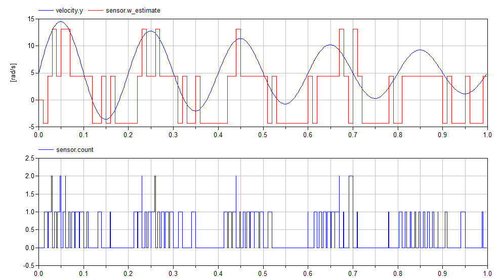
A similar effect can be observed if the rotational speed is low (relative to the number of teeth and the sample rate):

Pulse to Pulse Interval

The other approach to measuring rotational speed involves measuring the time between pulses. This can be done with the following model:

within Sensors.RotarySpeed;
model IntervalTime "Estimate speed by measuring interval between 'pip' signals"
  extends Sensors.Interfaces.RotarySpeedSensor;
  parameter Integer teeth "Number of teeth";
protected
  parameter Modelica.SIunits.Angle tooth_angle = Modelica.Constants.pi*2/teeth;
  Modelica.SIunits.Angle next_angle;
  Modelica.SIunits.Time last_time;
algorithm
  when initial() then
    next_angle := angle+tooth_angle-mod(angle,tooth_angle);
    w_estimate := 0;
    last_time := time;
  end when;
  when {angle>next_angle,
        angle<next_angle-tooth_angle,
        angle<next_angle-2*tooth_angle} then
    if time>pre(last_time) then
       next_angle := angle+tooth_angle;
       last_time := time;
       w_estimate :=tooth_angle/(time - pre(last_time));
    end if;
  end when;
end IntervalTime;

Using this sensor, we get the following estimate for rotational speed:

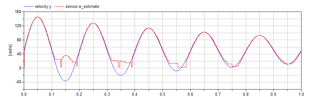
Comparison

The ToothCounter sensor model has the advantage (in hardware), that a simple circuit can be used to count the teeth and no higher level processing is really required except at the sample rate. In contrast, if we make our estimates based on the interval time, we need to make accurate and precise measurements of the interval time and act on them immediately (presumably forcing some kind of interrupt driven calculation).

The following figure shows the differences in the estimation error between the two approaches:

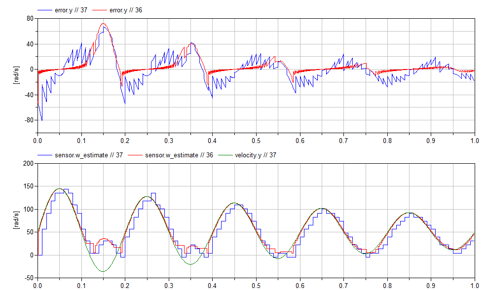
The plot on the top compares the error of both estimation methods. Blue is the error from the ToothCounter estimator and the red is the IntervalTime estimator. As we discussed before, using interval time gives us a more accurate estimation, but potentially requiring more expensive hardware. The bottom figure shows the estimated velocities against the reference signal (green). Once again, blue is the ToothCounter signal and red is the IntervalTime signal.

Conclusions

Clearly the accuracy of each approach depends on the design characteristics of the sensor and the range of speeds to be measured. In practice, different types of sensors require different kinds of electronics which also affect their feasibility for different applications.

But part of any model based system engineering approach to decide between sensors is to understand how these tradeoffs will affect system performance. And that means having to build models of the sensors that accurately capture the effects so a valid comparison can be made. For those who are interested, I discuss this topic in greater depth in Chapter 7 of my book.

Hopefully this post gives you some insight into how such models would be built in Modelica.